tw-rl

I will attempt to explain the basic idea of how diffusion models work! ... in only 15 tweets! 😲 Let's get started ↓

Diffusion models are *generative* models, which simply means given some example datapoints (your training dataset), generate more like it. For example, given cute dog images, generate more cute dog images! (1/15)

There are many generative models. GANs (like the ones powering http://thispersondoesnotexist.com ) are image generative models, GPT-3 is also a generative model, but for text. So just keep in mind that while we'll talk about images, the general principles can apply to other domains. (2/15)

Okay, an important idea of generative modeling is the idea of a data distribution. This simply describes how likely some datapoint is to be observed in reality. It's represented in math as p(x) (3/15)

Therefore, images that are likely to be observed have high p(x) (x represents the images) and images that are not common/weird/has artifacts/messed up have low p(x). (4/15)

Now if you want to generate new datapoints, you could either: 1. approximately model p(x) and sample from it - VAEs do this 2. model an approximate sampling function of p(x) but not p(x) itself - GANs do this Diffusion models propose an alternative approach! (5/15)

What if you knew how changing your datapoint x changes its probability of being observed p(x)? This rate of change is the derivative/gradient of p(x), written as ∇p(x). If you knew ∇p(x) then you could start at a random point & *iteratively* update it following ∇p(x) (6/15)

The question is how can we determine these gradients? We don't know p(x) so how could we get the ∇p(x)? We model it by training a neural network! This neural network will estimate ∇p(x) which we can use in an iterative sampling scheme. (7/15)

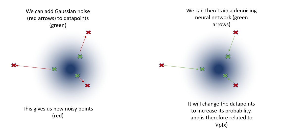
But how do we train a neural network to estimate ∇p(x)? The following insight helps: if we add random noise to a datapoint, it results in a datapoint with lower probability, because images with random noise are unlikely to be observed (8/15)

Then you can train a model to denoise noisy images by predicting the noise you need to remove. By subtracting out the predicted noise you're making the image a more likely datapoint, i.e. increasing p(x). You can imagine it's closely related to the rate of change ∇p(x) (9/15)

It can be proven mathematically that "noise prediction" is equivalent to predicting ∇ log p(x), termed as the score in statistics literature. Also, mathematically it's simpler to use the score instead of ∇p(x) for iterative sampling (10/15)

However if you look carefully above you might notice that this denoising approach gives the score for the noisy distribution & not the actual distribution! The idea is instead to denoise at multiple noise levels & as you iteratively sample the noise level is decreasing. (11/15)

One minor detail: the model is given the noise level as an input & sampling is carefully designed so that the noise level is known. The noise level tells the model approximately how much noise it needs to remove but the model needs to figure out the exact noise to remove. (12/15)

Image diffusion models are usually neural networks with the "U-net" architecture. It is a common arch. when going from one image to another, in this case iteratively going from an image to noise that we subtract out, effectively following ∇ log p(x) for our sampling. (13/15)

Here is an example of the sampling procedure. You can see how it starts out with random noise but the denoiser neural network iteratively subtracts out noise (which we said is equivalent to increasing p(x)) until we get a nice generated image!

And that's the basic idea of diffusion models! 1. Training a denoiser neural network for different levels of noise added to the images 2. Since the denoising is equivalent to learning the score, we take a random datapoint and iteratively update it with the learned score (15/15)

If you want to explore this further, check out the @fastdotai lectures where Jeremy Howard explores this in a little more detail than a Twitter thread 😅 https://www.fast.ai/posts/part2-2022-preview.html

Also, some of the diagrams here were taken by this awesome blog post by @YSongStanford which talks about diffusion models (sometimes also called score-based generative modeling, for reasons I hope you can see 😉) https://yang-song.net/blog/2021/score/

Next time, I'll attempt to explain some of the actual mathematical details of Denoising Diffusion Probabilistic Models (DDPM), the seminal paper published in 2020, as well as how these models are implemented in code!

If you found this thread useful, please like and retweet. Also consider following me to stay tuned (@iScienceLuvr)🙂